Lesson 8: Observability

A reference-style deep dive into metrics, logs, traces, SLOs, alerting — knowing what your system is doing. Read this as an article, not a transcript. The accompanying audio is the spoken companion; the article below is the canonical written reference.

Audience. Engineers designing, building, or operating distributed systems who want a clear mental model rather than a checklist of tools.

Prerequisites. Working knowledge of HTTP, basic SQL, and the idea of running more than one server behind a load balancer.

Table of contents

1. Why observability matters
2. The core mental model and where to start 3-12. In-depth sections below (see "Lesson body")

Lesson diagram

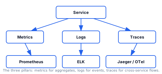
Figure 1. The canonical observability topology and control flow covered in this lesson.

1. Why observability matters

You cannot operate what you cannot see. Observability is the discipline of making a system's internal state understandable from its external outputs. The three pillars — metrics, logs, and traces — answer different questions. Knowing when to reach for each is the foundation.

The shift from "monitoring" to "observability" reflects a deeper truth: in a microservices system, you cannot pre-define every question you will need to ask. You need raw data (high-cardinality metrics, structured logs, distributed traces) and tools that can answer novel questions on the fly.

2. The three pillars

Metrics

Numeric values aggregated over time. Counters, histograms, summaries.

from prometheus_client import Counter, Histogram
requests_total = Counter('http_requests_total', 'Total HTTP requests', ['method', 'path', 'status'])
request_duration = Histogram('http_request_duration_seconds', 'Request duration', buckets=[0.01, 0.05, 0.1, 0.5, 1, 5])

@request_duration.time()
def handle_request(req):
    requests_total.labels(method=req.method, path=req.path, status='200').inc()
    return process(req)

Properties:

• Cheap to store (one number per metric per time interval).
• Easy to aggregate and alert on.
• Cannot tell you about individual events.

Logs

Discrete events with structured context.

import structlog
logger = structlog.get_logger()

logger.info("order_placed",
            order_id=42,
            total_cents=9999,
            user_id="user_123",
            latency_ms=234)

Properties:

• Per-event context (you can find the specific request that failed).
• Structured (JSON or key-value) is queryable; unstructured (free text) is not.
• Expensive at high volume; sample or aggregate for high-throughput services.

Traces

Causal chains of operations across services.

from opentelemetry import trace
tracer = trace.get_tracer(__name__)

with tracer.start_as_current_span("charge_order"):
    charge_payment(amount=99.99)
    with tracer.start_as_current_span("send_receipt"):
        send_email(...)

Properties:

• Show the path of a request through the system.
• Reveal where time was spent (which service, which span).
• Span context (trace ID, span ID) propagates through HTTP headers, gRPC metadata, message headers.

3. The four golden signals

Google SRE's four golden signals: every service should track these.

Latency

How long requests take. Track p50, p95, p99 — not just average.

# p99 latency over 5 minutes
histogram_quantile(0.99, rate(http_request_duration_seconds_bucket[5m]))

Traffic

How much demand is placed on the service. Requests per second.

rate(http_requests_total[5m])

Errors

Rate of requests failing. 4xx and 5xx counted separately.

rate(http_requests_total{status=~"5.."}[5m])

Saturation

How "full" the service is. CPU utilization, queue depth, connection pool occupancy.

100 - (avg by(instance) (rate(node_cpu_seconds_total{mode="idle"}[5m])) * 100)

4. RED method — for request-driven services

For every service, track:

• Rate — requests per second.
• Errors — failures per second.
• Duration — latency distribution.

# RED dashboard for "orders" service
sum(rate(http_requests_total{service="orders"}[5m]))    # rate
sum(rate(http_requests_total{service="orders",status=~"5.."}[5m]))  # errors
histogram_quantile(0.99, sum by(le) (rate(http_request_duration_seconds_bucket{service="orders"}[5m])))  # duration

5. USE method — for resources

For every resource (CPU, memory, disk, network):

• Utilization — percentage of time the resource is busy.
• Saturation — amount of work queued.
• Errors — error count.

Useful for infrastructure-level debugging (which machine is hot, which disk is filling).

6. SLOs, SLIs, and error budgets

SLO (Service Level Objective)

The target reliability. "99.9% of requests succeed in <500ms, measured over 30 days."

SLI (Service Level Indicator)

The measurement that backs the SLO. Successful-request ratio.

Error budget

The allowed failure rate over the SLO window. For a 99.9% SLO over 30 days:

total_seconds = 30 * 24 * 3600        # 2,592,000 seconds
budget = (1 - 0.999) * total_seconds   # 2,592 seconds of allowed downtime

The error budget is the team's spendable resource. Risky deploys consume it; if you exhaust it, you stop risky deploys and focus on reliability.

7. Alerting on SLOs

The point of SLOs is to drive alerts. The simplest alert: page when you are consuming error budget too fast.

# Alert if 2x burn rate over 1 hour
(
  sum(rate(http_requests_total{status=~"5.."}[1h]))
  / sum(rate(http_requests_total[1h]))
) > (2 * (1 - 0.999))   # 2x the SLO failure rate

Burn-rate alerts are more useful than threshold alerts: they catch sustained problems early without paging on transient blips.

# Prometheus alert
- alert: HighErrorBudgetBurn
  expr: |
    sum(rate(requests_failed[5m])) / sum(rate(requests_total[5m])) > (2 * 0.001)
  for: 5m
  labels:
    severity: page
  annotations:
    summary: "Error budget burning 2x faster than planned"

8. Distributed tracing deep dive

A trace is a tree of spans. Each span represents a unit of work; spans have a name, start/end time, attributes, and a parent.

# Span structure
trace: abc123
  span: receive_request (root)
    span: validate_input
    span: call_database
    span: call_payment_service
      span: build_request
      span: send_http_request
      span: parse_response

The trace ID is propagated as a header (W3C traceparent) across every service boundary.

Sampling

Tracing every request is expensive. Sample:

# Tail-based sampling (keep all error traces; sample 1% of success)
def should_sample(trace):
    if trace.has_error():
        return True
    return random.random() < 0.01

Tail-based sampling is better than head-based: it keeps the interesting traces and discards the boring ones.

9. Structured logging best practices

# Good: structured, queryable
logger.info("order_placed", order_id=42, total=99.99, user_id="user_123")

# Bad: unstructured string
logger.info(f"order placed: id=42 total=99.99 user=user_123")

Rules:

• Use JSON or key-value. Free text is not queryable.
• Include request ID. Every log line in a request shares an ID; you can grep by it.
• Avoid PII. No email addresses, no credit card numbers.
• Log levels matter. ERROR = page; WARN = investigate; INFO = default; DEBUG = troubleshooting.

10. Cardinality — the silent killer

A metric with high-cardinality labels explodes the number of time series.

# Bad: user_id as a label creates millions of series
requests_total.labels(user_id=req.user_id).inc()

# Good: bounded labels (status, region, method)
requests_total.labels(method=req.method, status=resp.status, region=req.region).inc()

Cardinality budget:

• Status code: 5 values (200, 4xx, 5xx, etc.).
• Region: 5-20 values.
• HTTP method: 4 values (GET, POST, PUT, DELETE).
• Path template: /orders/{id}, not /orders/42, /orders/43, ...

Stick to bounded cardinality. The rule of thumb: a metric label set should have < 1000 unique combinations.

11. Dashboards that matter

A good dashboard answers the questions you ask during incidents. Three layers:

1. Overview — service health at a glance (RED metrics + SLO compliance).
2. Drill-down — per-endpoint latency, per-shard traffic.
3. Dependencies — downstream service health, queue depths.

The worst dashboards are vanity dashboards (CPU, memory, network) without application context. CPU is not a problem until it is; latency is a problem the moment it spikes.

12. OpenTelemetry — the standard

OpenTelemetry (OTel) is the vendor-neutral standard for metrics, logs, and traces. It merges OpenCensus and OpenTracing into one API/SDK.

from opentelemetry import trace
from opentelemetry.sdk.trace import TracerProvider
from opentelemetry.sdk.trace.export import BatchSpanProcessor
from opentelemetry.exporter.otlp.proto.grpc.trace_exporter import OTLPSpanExporter

provider = TracerProvider()
provider.add_span_processor(BatchSpanProcessor(OTLPSpanExporter(endpoint="http://otel-collector:4317")))
trace.set_tracer_provider(provider)

One instrumentation, many backends (Jaeger, Tempo, Datadog, Honeycomb). Switching backends does not require re-instrumentation.

13. Key takeaways

• Metrics, logs, traces answer different questions — use all three.
• Track the four golden signals for every service: latency, traffic, errors, saturation.
• SLOs drive alerts; burn-rate alerts catch real problems without alert fatigue.
• Structured logs are queryable; unstructured logs are not.
• High-cardinality labels are a budget; respect it.
• Sample traces intelligently; tail-based sampling keeps the interesting ones.
• OpenTelemetry is the standard; one instrumentation, many backends.

Appendix: terms

• SLI — Service Level Indicator (the measurement).
• SLO — Service Level Objective (the target).
• Error budget — the allowed failure rate over the SLO window.
• Burn rate — how fast you are consuming the error budget.
• Span — a unit of work within a trace.
• Cardinality — the number of unique values a metric label can take.
• Tail-based sampling — sampling decision made after the trace is complete.

Appendix: source dialogue excerpt

The audio for this lesson was synthesized from the following Cantonese dialogue (verbatim, not translated):

• M: 各位同學早晨, 我係子謙。歡迎收聽系統架構課程第八課, 亦都係 series 嘅最後一課。今日嘅主題係 Observability 同 SRE 嘅 practice。…
• F: 大家好, 我係曉晴。Observability 唔止係 log metric trace, 包括 SLO 設計, alerting strategy, 同 incident response 嘅 best practice。今日我哋會拆解 SRE 嘅 discipline, 包括 error budget, blame…
• M: 首先講解基本概念。Observability 嘅 core 係 unknown unknowns, 即係你唔知道 production 會出咩事, 所以你嘅 monitoring 必須 generic, 可以 debug 任何問題。傳統 monitoring 係 known unknowns, 即係 monitor k…
• F: Observability 嘅三個 pillar, 即係 log, metric, trace。Log 即係 discrete event record, 例如某個 request 失敗, 包含 timestamp, trace id, error message。Metric 即係 numeric time seri…
• M: 好, 第一個 important concept 係 SLO 即係 Service Level Objective。SLO 係 reliability 嘅 target, 例如百分之九十九點九 availability 即係每月 downtime 少過四十三分鐘。SLO 唔係 SLA, SLA 即係 Service L…
• F: SLO 嘅 design 必須 measurable, 即係有 metric 可以 track。常見嘅 SLO 包括 availability, 即係 successful request 嘅 percentage。Latency, 即係 P99 response time 少過 N 毫秒。Throughput, 即係…

Full dialogue contains 34 segments; see script_raw.json in the source folder.